2. Results
2.1. Correlation function
We show that computing the 3d correlation function \(\xi(r)\) from the 3d
power spectrum \(P(k)\) works. This is implemented in the
corfu.ptoxi() function, using the FFTLog algorithm.
First, we import a number of required packages. We will need the special
functions hyp2f1 and gamma.
import numpy as np
import matplotlib.pyplot as plt
from scipy.special import hyp2f1, gamma
For testing, we will define a 3d power spectrum \(P(k) = k^a \, e^{-bk}\) where \(a\) and \(b\) are arbitrary positive parameters. We set up a grid of wavenumbers \(k\) over which we evaluate the power spectrum.
k = np.logspace(-2, 2, 1000)
We fix the values of the parameters \(a\) and \(b\).
a, b = 2.0, 0.5
Finally, we are able to compute the input 3d power spectrum.
p = k**a*np.exp(-b*k)
The basic setup is complete. We now use corfu to convert the 3d power
spectrum to a 3d correlation function.
import corfu
The computation is done with the corfu.ptoxi() function. Here, we compute
\(\xi(r)\) for the exact (non-Limber) projection. The FFTLog bias parameter
\(q = 1.0\) is chosen to improve the result while not causing numerical
issues.
r, xi_ptoxi = corfu.ptoxi(k, p, q=1.0, limber=False)
The true 3d correlation function is the integral (1.17), which we can evaluate analytically for our sample power spectrum,
Using the \(r\) values that the call to corfu.ptoxi() returned, the
truth values are readily computed using SciPy’s gamma
function:
xi_truth = (r**2+b**2)**(-(a+2)/2)*gamma(a+2)*np.sin((a+2)*np.arctan(r/b))/(2*np.pi**2*r)
We repeat the steps for Limber’s correlation function \(\xi_{\rm L}(r)\),
which is returned by corfu.ptoxi() when setting limber=True:
r_L, xi_L_ptoxi = corfu.ptoxi(k, p, q=1.0, limber=True)
The analytical results for Limber’s correlation function (1.27) can similarly be obtained,
where \(_2F_1(a, b; c; z)\) is the hypergeometric function, available
through SciPy’s scipy.special.hyp2f1:
xi_L_truth = b**(-a-2)*gamma(a+2)*hyp2f1((a+2)/2, (a+3)/2, 1, -(r_L/b)**2)/(2*np.pi*r_L)
The results of the comparison are shown in Fig. 2.1. It is clear
that corfu.ptoxi() produces the desired output, up to aliasing due to the
circular nature of the underlying FFTLog transform.
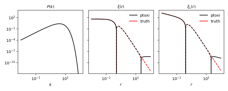
Fig. 2.1 Computing the 3d correlation function \(\xi(r)\) and Limber’s correlation function \(\xi_{\rm L}(r)\) from the 3d power spectrum \(P(k)\) using corfu.ptoxi().